Plot for kernel density estimate

Plot for kernel density estimate for 1- to 3-dimensional data.

Usage

# S3 method for class 'kde'
plot(x, ...)

Arguments

x

object of class kde (output from kde)

...

other graphics parameters:

display: type of display, "slice" for contour plot, "persp" for perspective plot, "image" for image plot, "filled.contour" for filled contour plot (2-d); "plot3D", "rgl" (3-d)
cont: vector of percentages for contour level curves
abs.cont: vector of absolute density estimate heights for contour level curves
approx.cont: flag to compute approximate contour levels. Default is FALSE.
col: plotting colour for density estimate (1-d, 2-d)
col.cont: plotting colour for contours
col.fun: plotting colour function for contours
col.pt: plotting colour for data points
colors: vector of colours for each contour (3-d)
jitter: flag to jitter rug plot (1-d). Default is TRUE.
lwd.fc: line width for filled contours (2-d)
xlim,ylim,zlim: axes limits
xlab,ylab,zlab: axes labels
add: flag to add to current plot. Default is FALSE.
theta,phi,d,border: graphics parameters for perspective plots (2-d)
drawpoints: flag to draw data points on density estimate. Default is FALSE.
drawlabels: flag to draw contour labels (2-d). Default is TRUE.
alpha: transparency value of plotting symbol
alphavec: vector of transparency values for contours (3-d)
size: size of plotting symbol (3-d).

Value

Plots for 1-d and 2-d are sent to graphics window. Plot for 3-d is sent to graphics/RGL window.

Details

For kde objects, the function headers for the different dimensional data are


  ## univariate
  plot(fhat, xlab, ylab="Density function", add=FALSE, drawpoints=FALSE, col=1,
       col.pt=4, col.cont=1, cont.lwd=1, jitter=FALSE, cont, abs.cont,
       approx.cont=TRUE, alpha=1, ...)

  ## bivariate
  plot(fhat, display="slice", cont=c(25,50,75), abs.cont, approx.cont=TRUE,
       xlab, ylab, zlab="Density function", cex=1, pch=1, add=FALSE,
       drawpoints=FALSE, drawlabels=TRUE, theta=-30, phi=40, d=4, col.pt=4,
       col, col.fun, alpha=1, lwd=1, border=1, thin=3, kdde.flag=FALSE,
       ticktype="detailed", ...)

  ## trivariate
  plot(fhat, display="plot3D", cont=c(25,50,75), abs.cont, approx.cont=TRUE,
       colors, col, col.fun, alphavec, size=3, cex=1, pch=1, theta=-30, phi=40,
       d=4, ticktype="detailed", bty="f", col.pt=4, add=FALSE, xlab, ylab,
       zlab, drawpoints=FALSE, alpha, box=TRUE, axes=TRUE, ...)

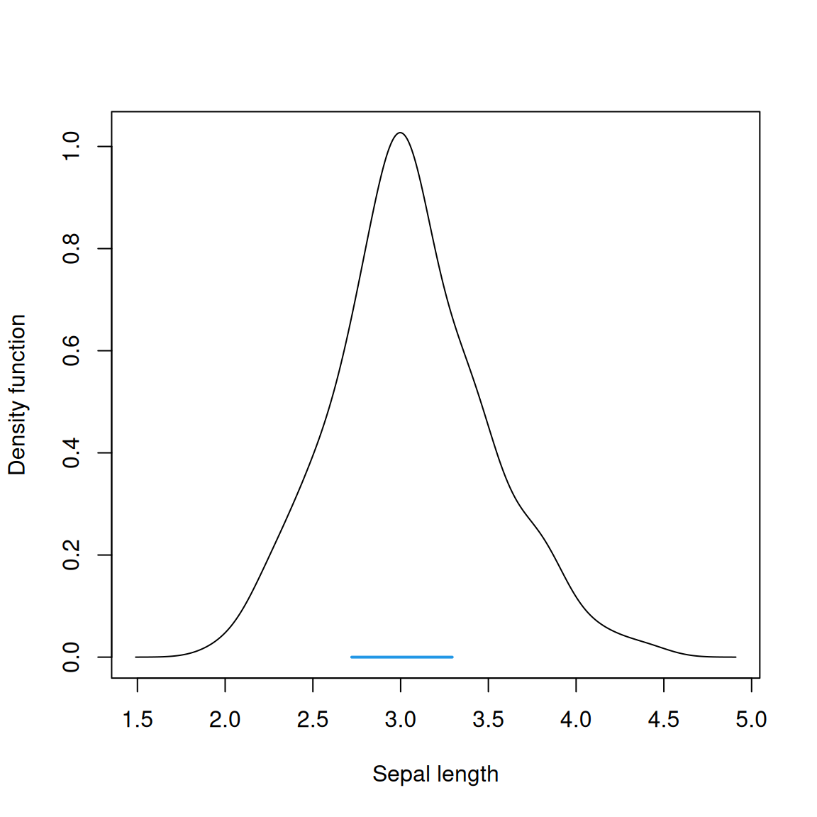
For 1-dimensional data, the plot is a standard plot of a 1-d curve. If drawpoints=TRUE then a rug plot is added. If cont is specified, the horizontal line on the x-axis indicates the cont% highest density level set.

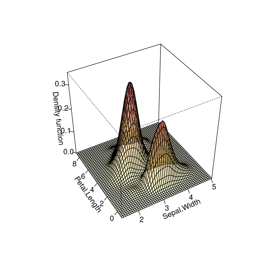
For 2-dimensional data, the different types of plotting displays are controlled by the display parameter. (a) If display="slice" then a slice/contour plot is generated using contour. (b) If display is "filled.contour" then a filled contour plot is generated. The default contours are at 25%, 50%, 75% or cont=c(25,50,75) which are upper percentages of highest density regions. (c) If display="persp" then a perspective/wire-frame plot is generated. The default z-axis limits zlim are the default from the usual persp command. (d) If display="image" then an image plot is generated.

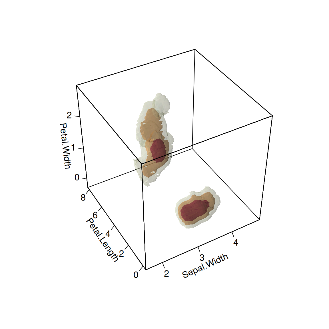
For 3-dimensional data, the plot is a series of nested 3-d contours. The default contours are cont=c(25,50,75). The default opacity alphavec ranges from 0.1 to 0.5. For ks \(\geq\) 1.12.0, base R graphics becomes the default plotting engine: to create an rgl plot like in previous versions, set display="rgl".

To specify contours, either one of cont or abs.cont is required. cont specifies upper percentages which correspond to probability contour regions. If abs.cont is set to particular values, then contours at these levels are drawn. This second option is useful for plotting multiple density estimates with common contour levels. See contourLevels for details on computing contour levels. If approx=FALSE, then the exact KDE is computed. Otherwise it is interpolated from an existing KDE grid, which can dramatically reduce computation time for large data sets.

If a colour function is specified in col.fun, it should have the number of colours as a single argument, e.g. function(n){hcl.colors(n, ...)}. The transparent background colour is automatically concatenated before this colour function. If col is specified, it overrides col.fun. There should be one more colour than the number of contours, i.e. background colour plus one for each contour.

Examples

## univariate example
data(iris)
fhat <- kde(x=iris[,2])
plot(fhat, cont=50, col.cont=4, cont.lwd=2, xlab="Sepal length")


## bivariate example
fhat <- kde(x=iris[,2:3])
plot(fhat, display="filled.contour", cont=seq(10,90,by=20), lwd=1, alpha=0.5)

plot(fhat, display="persp", border=1, alpha=0.5)


## trivariate example
fhat <- kde(x=iris[,2:4])
plot(fhat)

if (interactive()) plot(fhat, display="rgl")