As a compromise then, the most computationally intensive functions can be written in C (which is a more efficient programming language) to improve performance and leaving the rest of the (non-performance critical) functions in Splus/ R. The C code is dynamically loaded at run-time and called by the appropriate Splus/ R functions. This way usability is maintained AND efficiency improved.
Now this is pretty much standard: what is different about this software is that it you can control amount and type of traffic assignment. By changing the amount and type of reassignment, you can run simulations in much less time. There are two types of reassignment:
Please note that a label correcting algorithm is used here to find the shortest paths. This particular form of the algorithm uses the 'forward star' form of a network. Please see Urban Transportation Networks by Sheffi for further details.
assign.path - assigns shortest paths to all travellers
change.cost - change BPR cost parameters or standard deviation for a link
plot.flow.hist - plot flow history for one link
plot.network - plot current flows for entire network
prepare.network - prepares the network, demand, node co-ordinates and memory weights
total.mean - computes the totals and mean link flow and total cost?????
prepare.network is used first before
change.cost and assign.path can be used.
The remaining functions (...) are used after assign.path has completed.
prepare.networkprepare.network then converts the network to its forward star form, the
demand and node-coordinate matrices into lists. The function header is
prepare.network(network, demand, node.coord, memory)It takes the network, demand matrix, node coordinate matrix and the memory weights and returns a list of the appropriate data structures which is henceforth called the network specification.
assign.pathassign.path to assign travellers their minimum cost or shortest paths. The function header is (with the default values)
assign.path(net.spec, err = 'a', n.iter = 100, graph = 'n', scale = 100,
    save.name = "save", default.init = 'y', spath.table.init,
    flow.mem.init, append = 'n', flow.hist.init, thresh = 100, ...)
where
net.spec - network specification
err - type of error structure
n.iter - no. of iterations
thresh - threshold for implicit reassignment (default = 100)
graph
scale - line width in plot = 1 + flow/ scale (default = 100)
save.name - filename where output is saved (default = "save.Rdata")
default.init spath.table.init - initial (user-specified) shortest paths
flow.mem.init - initial (user-specified) link flows
append
flow.hist.initflow.hist.init - initial (user-specified) flow history
flow.hist - link flow history (ie flows for all links for all iterations)
spath.table - shortest paths taken by each travellerflow.mem - previous n_W link flows
cost.mem - previous n_W measured costs
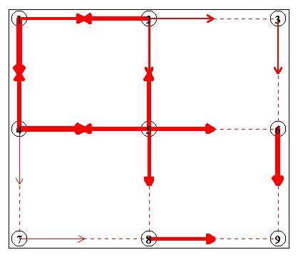
plot.networkgraph is equal to 'y' is assign.path then a plot of the
flow for each iteration is shown. This is recommended as it helps visualise the data
and it doesn't decrease the speed of the simulation significantly. The graph has the
following features
If graph = 'n' then a message is printed in the command line stating which iteration the function is up to.
The function header is
plot.network(net.spec, scale = 100, flow, ...)where
net.spec - network specification
scale - line width in plot = 1 + flow/ scale (default = 100)
flow - link flows (from one iteration) to be plotedplot.flow.histassign.path) of a particular link.
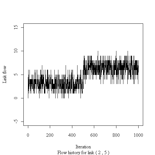
The function header is
plot.flow.hist(net.spec, link, flow.hist,...)where
net.spec - network specification
link - link in the form of (from node, to node) eg. c(1, 5) is
the link from node 1 to node 5
flow.hist - link flow history
change.costchange.cost(net.spec, link, const.new = NULL, coeff.new = NULL,
power.new = NULL, sd.new = NULL)
net.spec - network specification
link - link eg. c(1, 5)
const.new - new BPR constant parameter
coeff.new - new BPR floe coefficient parameter
power.new - new BPR power parameter
const.new - new standard deviation
total.meantotal.mean(net.spec, flow.hist, ...)where
net.spec - network specification
flow.hist - flow history
cost.tot - total cost on network
cost.mean - mean total cost on network
flow.tot - total link flow on network
flow.mean - mean link flow on network
On the 501st day, road works on link (1, 4) closes it off to traffic (in the south direction only). After another 500 iterations, the flow is shown below. Note that he traffic that used to flow on link (1,4) is now diverted to link (1, 2):
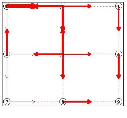
The first 500 iterations took 94 s on a Celeron 550 MHz PC. The second 93 s. As there were 20 travellers in total, this equates to 10000 shortest paths.
| Proportion of reassignment | |||
| Threshold | 1 | 0.5 | 0.2 |
| 100 | 1454 s 426.42 |
1007 s 427.15 |
557 s 429.47 |
| Infinite | 2754 s 427.05 |
1452 s 423.02 |
571 s 429.86 |
.dll file extension.
The C compiler used was LCC Win32 - it is available free on the Internet. It is pretty nifty in that it can create DLLs in a single integrated project. I have also included instructions that can be used to create DLLs manually - these instructions can be easily(?) adapted to other C compilers.
file.
By default, LCC Win32 expects that the source file is called file.c and will create a DLL called file.dll. Next, on the "Definition of a new project" screen, remember to click the radio button for the dynamic link library in the bottom right hand corner. Select the directories where LCC Win32 expects input and output.
__declspec(dllexport)
should be added to the function declaration to prompt the C compiler to export it. For example if the usual function declaration is
void hello(int *world)then the exporting version is just
void __declspec(dllexport) hello(int *world)Note:
__declspec(dllexport)
void
int *).
file.obj and export file file.exp (this second file contains all the names of the exported functions).
dll.tpl file (found in, say, C:\lcc\lib\wizard) before the actual function code.
For each function that you want to export (make visible) to Splus/ R,
__declspec(dllexport) should be added to the function declaration
to prompt the C compiler to export it. For example if the usual function declaration is
void hello(int world)then the exporting version is just
void __declspec(dllexport) hello(int *world)Note:
__declspec(dllexport)
void
int *).
#include <windows.h>
autoexec.bat e.g.
SET PATH = %PATH%; C:\LCC\BINif the LCC Win32 binary
.exe file is in the directory
C:\LCC\BIN
(This only needs to be done once and you may need to
restart your computer for Windows to
update the PATH variable).
file.c is. The following commands will produce a DLL.
lcc file.c
lcclnk -dll file.obj
file.obj and export file file.exp
(this contains all the names of the exported functions).
file.c simply type in the command
line R CMD SHLIB file.cThis will automatically create the object file (
file.o) and the
shared library (file.so). Then just run R as usual.
Splus5 CHAPTERin the command line, in the directory where
file.c is. Then type
in Splus5 makewhich creates the shared library (S.so) as well as the makefile (
makefile) and the object file
(file.o). Please see the page by the
Ohio State University
Statistics Department for more details.
dyn.load is used to dynamically load the DLL
.C is used to call the C function in the DLL
file.dll then use
dyn.load("C:\myfiles\file.dll")
If the C function name is hello then in the file.exp
it's known as _hello. This underscore is important! To check that
hello has been loaded use
is.loaded(symbol.C("_hello"))
Suppose the C function is hello(int *world) and that it increments the value
of the world parameter. Then to call this function in Splus/ R:
world <- 5
.C(symbol.C("_hello"), as.integer(world))
returns
[[1]]
6
Hence, when using
.C, a list of the modified values of all
parameters that are passed into a C function is returned to Splus/ R.
To ensure that any difference between Splus/R and C in storing variables are correctly converted, use the correspondence outlined in the table below (adapted from Venables & Ripley and Writing R Extensions).
| Splus/ R storage mode | C type |
"logical"
|
long *, int *
|
To dynamically unload any loaded shared libraries, just use
dyn.unload("C:\myfiles\file.dll")
dyn.load is used to dynamically load the DLL
.C is used to call the C function in the DLL
file.so then use
dyn.load("file.so")
To check that
hello has been loaded use
is.loaded(symbol.C("hello"))
Note there is no underscore like in Windows.
Suppose the C function is hello(int *world) and that it increments the value
of the world parameter. Then to call this function in Splus/ R:
world <- 5
.C(symbol.C("hello"), as.integer(world))
returns
[[1]]
6
Hence, when using
.C, a list of the modified values of all
parameters that are passed into a C function is returned to Splus/ R.
The type casting applies in the same way as for Windows.
To dynamically unload any loaded shared libraries, just use
dyn.unload("file.so")
Venables, W. N. & Ripley, B. D. (1994) Modern Applied Statistics with S-Plus (2nd ed.) New York: Springer Verlag.
R Development Core Team (2000) Writing R Extensions http://cran.r-project.org
Becker, R. A., Chambers J. M., Wilks, A. R. (1988) The New S Language California: Cole Advanced Books & Software.
Navia, J. (1998) LCC-Win32 User's Manual https://lcc-win32.services.net
Roncalli, T. (?) Creating DLLs for GAUSS Using LCC-Win32 http://www.thierry-roncalli.com/Gauss.html
Sheffi, (1985) Urban Transportation Networks Englewood Cliffs: Prentice-Hall.
Department of Statistics, The Ohio State University, (?) Dynamic Loading in Splus http://www.stat.ohio-state.edu/department/docs/statpack/dynload.html