Kernel density based local two-sample comparison test

Kernel density based local two-sample comparison test for 1- to 6-dimensional data.

Usage

kde.local.test(x1, x2, H1, H2, h1, h2, fhat1, fhat2, gridsize, binned, 
   bgridsize, verbose=FALSE, supp=3.7, mean.adj=FALSE, signif.level=0.05,
   min.ESS, xmin, xmax)

Arguments

x1,x2: vector/matrix of data values
H1,H2,h1,h2: bandwidth matrices/scalar bandwidths. If these are missing, Hpi or hpi is called by default.
fhat1,fhat2: objects of class kde
binned: flag for binned estimation
gridsize: vector of grid sizes
bgridsize: vector of binning grid sizes
verbose: flag to print out progress information. Default is FALSE.
supp: effective support for normal kernel
mean.adj: flag to compute second order correction for mean value of critical sampling distribution. Default is FALSE. Currently implemented for d<=2 only.
signif.level: significance level. Default is 0.05.
min.ESS: minimum effective sample size. See below for details.
xmin,xmax: vector of minimum/maximum values for grid

Value

A kernel two-sample local significance is an object of class kde.loctest which is a list with fields:

fhat1,fhat2: kernel density estimates, objects of class kde
chisq: chi squared test statistic
pvalue: matrix of local \(p\)-values at each grid point
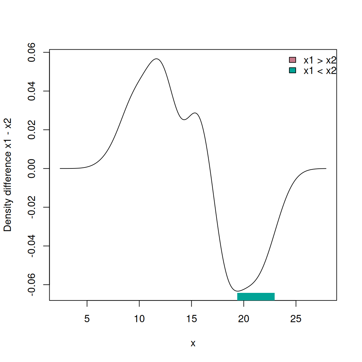
fhat.diff: difference of KDEs
mean.fhat.diff: mean of the test statistic
var.fhat.diff: variance of the test statistic
fhat.diff.pos: binary matrix to indicate locally significant fhat1 > fhat2
fhat.diff.neg: binary matrix to indicate locally significant fhat1 < fhat2
n1,n2: sample sizes
H1,H2,h1,h2: bandwidth matrices/scalar bandwidths

Details

The null hypothesis is \(H_0(\bold{x}): f_1(\bold{x}) = f_2(\bold{x})\) where \(f_1, f_2\) are the respective density functions. The measure of discrepancy is \(U(\bold{x}) = [f_1(\bold{x}) - f_2(\bold{x})]^2\). Duong (2013) shows that the test statistic obtained, by substituting the KDEs for the true densities, has a null distribution which is asymptotically chi-squared with 1 d.f.

The required input is either x1,x2 and H1,H2, or fhat1,fhat2, i.e. the data values and bandwidths or objects of class kde. In the former case, the kde objects are created. If the H1,H2 are missing then the default are the plug-in selectors Hpi. Likewise for missing h1,h2.

The mean.adj flag determines whether the second order correction to the mean value of the test statistic should be computed. min.ESS is borrowed from Godtliebsen et al. (2002) to reduce spurious significant results in the tails, though by it is usually not required for small to moderate sample sizes.

References

Duong, T. (2013) Local significant differences from non-parametric two-sample tests. Journal of Nonparametric Statistics 25, 635–645.

Godtliebsen, F., Marron, J.S. & Chaudhuri, P. (2002) Significance in scale space for bivariate density estimation. Journal of Computational and Graphical Statistics 11, 1–22.

Examples

data(crabs, package="MASS")
x1 <- crabs[crabs$sp=="B", 4]
x2 <- crabs[crabs$sp=="O", 4]
loct <- kde.local.test(x1=x1, x2=x2)
plot(loct)


## see examples in ? plot.kde.loctest