Plot for kernel local significant difference regions

Plot for kernel local significant difference regions for 1- to 3-dimensional data.

Usage

# S3 method for class 'kde.loctest'
plot(x, ...)

Arguments

x

object of class kde.loctest (output from kde.local.test)

...

other graphics parameters:

lcol

colour for KDE curve (1-d)

col

vector of 2 colours. First colour: sample 1>sample 2, second colour: sample 1<sample2.

add

flag to add to current plot. Default is FALSE.

rugsize

height of rug-like plot (1-d)

add.legend

flag to add legend. Default is TRUE.

pos.legend

position label for legend (1-d, 2-d)

alphavec

vector of transparency values for contour (3-d)

and those used in plot.kde

Value

Plots for 1-d and 2-d are sent to graphics window. Plot for 3-d is sent to graphics/RGL window.

Details

For kde.loctest objects, the function headers are

   ## univariate
   plot(x, lcol, col, add=FALSE, xlab="x", ylab, rugsize, add.legend=TRUE,
        pos.legend="topright", alpha=1, ...)

   ## bivariate
   plot(x, col, add=FALSE, add.legend=TRUE, pos.legend="topright", alpha=1,
        ...)

   ## trivariate
   plot(x, col, color, add=FALSE, box=TRUE, axes=TRUE, alphavec=c(0.5, 0.5),
        add.legend=TRUE, ...)

See also

kde.local.test

Examples

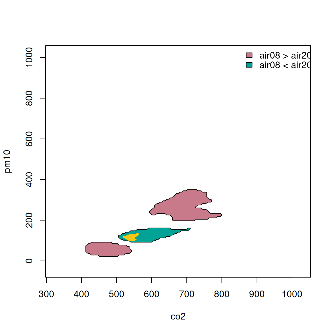
## bivariate
data(air)
air.var <- c("co2","pm10","no")
air <- air[, c("date","time",air.var)]
air2 <- reshape(air, idvar="date", timevar="time", direction="wide")
a1 <- as.matrix(na.omit(air2[, paste0(air.var, ".08:00")]))
a2 <- as.matrix(na.omit(air2[, paste0(air.var, ".20:00")]))
colnames(a1) <- air.var
colnames(a2) <- air.var
air08 <- a1[,c("co2","pm10")]
air20 <- a2[,c("co2","pm10")]

loct <- kde.local.test(x1=air08, x2=air20)
plot(loct, lwd=1)

## significant curvature regions
air20.fs <- kfs(air20)
plot(air20.fs, add=TRUE)


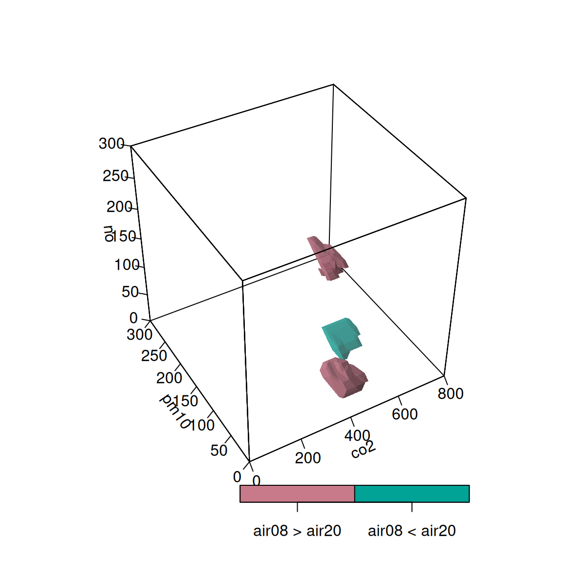
## trivariate
air08 <- a1; air20 <- a2
loct <- kde.local.test(x1=air08, x2=air20)
plot(loct, xlim=c(0,800), ylim=c(0,300), zlim=c(0,300))